Latitude hypothesis test
The following topics show the basic steps for testing the latitude
hypothesis using the entrainment model.
Hypothesis statement
Populations residing close to the equator (latitude 0°) (i.e., with greater average insolation) have, on average, a shorter duration/morning circadian period when compared to populations residing near the planet’s poles (i.e., with lower average insolation) (Leocadio-Miguel et al., 2017; Roenneberg et al., 2003).
In mathematical terms, this hypothesis can be written as follows:
The latitude hypothesis is based on the idea that regions located at latitudes close to the poles have, on average, a lower incidence of annual sunlight when compared to regions close to the equator (latitude 0°).
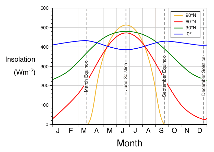
Monthly values of available insolation in Wm-2 for the equator (0°), 30°, 60°, and 90° North.
Figure credits: Pidwirny (2019).
Thus, it is understood by deduction that the regions close to the equator have a stronger solar zeitgeber, which, according to theory, should generate a greater propensity for synchronizing the circadian rhythms of these populations to the light-dark cycle, reducing the amplitude and the diversity of circadian phenotypes. This would also give these populations a morning characteristic when compared to populations living far from the equator, in which the opposite would occur, i.e., a greater amplitude and diversity of circadian phenotypes and an evening characteristic when compared to populations living near the equator. (Roenneberg et al., 2003).

Hypothetical distribution of chronotypes (circadian phenotypes) for populations exposed to a strong (black) solar zeitgeber and a weak (striped) zeitgeber based on mid-sleep phase.
Figure credits: Roenneberg et al. (2003).
1. Do the initial setup
import entrainment
2. Run the model for both groups
n = 10**3
lam_c = 3750
n_cycles = 3
repetitions = 10**2
x_name = "Nascente do rio Ailã"
y_name = "Arroio Chuí"
By season
North group (Location: Nascente do Rio Ailã) (Latitude: 5.272)
north_by_season = entrainment.run_model(
    n = n, labren_id = 72272, by = "season", lam_c = lam_c, n_cycles = n_cycles,
    repetitions = repetitions, plot = False, show_progress = False
    )
South group (Location: Arroio Chuí) (Latitude: -33.752)
south_by_season = entrainment.run_model(
    n = n, labren_id = 1, by = "season", lam_c = lam_c, n_cycles = n_cycles,
    repetitions = repetitions, plot = False, show_progress = False
    )
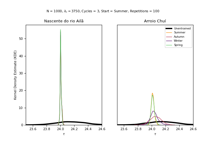
entrainment.plot_model_line_1_2(
    north_by_season, south_by_season, x_title = x_name, y_title = y_name
    )
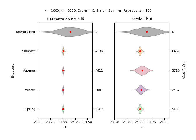
entrainment.plot_model_violin_1_2(
    north_by_season, south_by_season, x_title = x_name, y_title = y_name
    )
By year
North group (Location: Nascente do Rio Ailã) (Latitude: 5.272)
north_by_year = entrainment.run_model(
    n = n, labren_id = 72272, by = "year", lam_c = lam_c, n_cycles = n_cycles,
    repetitions = repetitions, plot = False, show_progress = False
    )
South group (Location: Arroio Chuí) (Latitude: -33.752)
south_by_year = entrainment.run_model(
    n = n, labren_id = 1, by = "year", lam_c = lam_c, n_cycles = n_cycles,
    repetitions = repetitions, plot = False, show_progress = False
    )
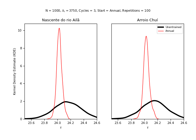
entrainment.plot_model_line_1_2(
    north_by_year, south_by_year, x_title = x_name, y_title = y_name
    )
3. Analyze the distributions of both groups
For more information about the values presented, see
scipy.stats.kstest()
and
scipy.stats.shapiro().
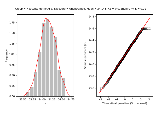
North group (Location: Nascente do Rio Ailã) (Latitude: 5.272)
Unentrained (Control)
stats = entrainment.analyze_model(
    model = north_by_season, exposure = "unentrained", name = x_name
    )
#> ---------------------------------------------------------
#>
#> [Group: Nascente do rio Ailã | Exposure: Unentrained]
#>
#> Mean = 24.148469728740682
#> Var. = 0.04081896119474018
#> SD = 0.20203702926627135
#>
#> Min. = 23.56882916499755
#> 1st Qu. = 24.01488782294597
#> Median = 24.148234332873688
#> 3rd Qu. = 24.29577424685605
#> Max. = 24.6
#>
#> Kurtosis = -0.32447057324198303
#> Skewness = -0.06893168079322273
#>
#> Kolmogorov-Smirnov test p-value = 0.0
#> Shapiro-Wilks test p-value = 0.009946780279278755
#>
#> ---------------------------------------------------------
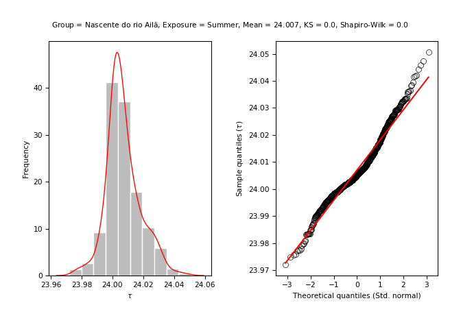
Summer
stats = entrainment.analyze_model(
    model = north_by_season, exposure = "summer", name = x_name
    )
#> ---------------------------------------------------------
#>
#> [Group: Nascente do rio Ailã | Exposure: Summer]
#>
#> Mean = 24.006999634122447
#> Var. = 0.00012367951240324957
#> SD = 0.01112112909749948
#>
#> Min. = 23.971999202966348
#> 1st Qu. = 24.00037498014924
#> Median = 24.005294156727402
#> 3rd Qu. = 24.012480086444633
#> Max. = 24.050759364023435
#>
#> Kurtosis = 0.954467089729472
#> Skewness = 0.542218351646886
#>
#> Kolmogorov-Smirnov test p-value = 0.0
#> Shapiro-Wilks test p-value = 2.853525927918113e-14
#>
#> ---------------------------------------------------------
Autumn
stats = entrainment.analyze_model(
    model = north_by_season, exposure = "autumn", name = x_name
    )
#> ---------------------------------------------------------
#>
#> [Group: Nascente do rio Ailã | Exposure: Autumn]
#>
#> Mean = 24.006421180918203
#> Var. = 0.00010496412004668206
#> SD = 0.01024519985391608
#>
#> Min. = 23.97441171192965
#> 1st Qu. = 24.00036012524516
#> Median = 24.004706190747772
#> 3rd Qu. = 24.011407636606492
#> Max. = 24.046190020477425
#>
#> Kurtosis = 1.0022899618902805
#> Skewness = 0.5642171633726051
#>
#> Kolmogorov-Smirnov test p-value = 0.0
#> Shapiro-Wilks test p-value = 7.410792052448597e-15
#>
#> ---------------------------------------------------------

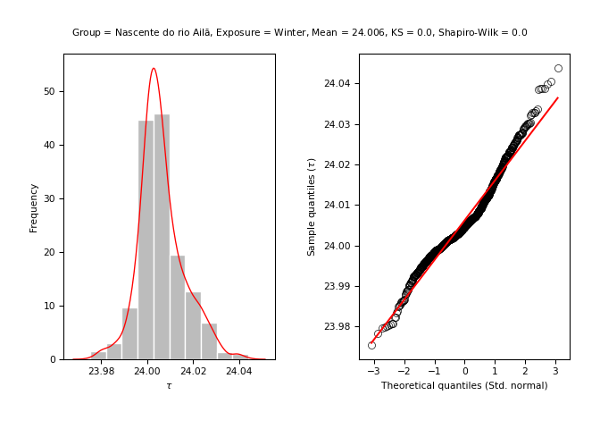
Winter
stats = entrainment.analyze_model(
    model = north_by_season, exposure = "winter", name = x_name
    )
#> ---------------------------------------------------------
#>
#> [Group: Nascente do rio Ailã | Exposure: Winter]
#>
#> Mean = 24.006179180043823
#> Var. = 9.583665584921525e-05
#> SD = 0.009789619801055364
#>
#> Min. = 23.97531283237005
#> 1st Qu. = 24.000383212627224
#> Median = 24.004636268415513
#> 3rd Qu. = 24.011182950769722
#> Max. = 24.04395631085106
#>
#> Kurtosis = 0.9914111157597341
#> Skewness = 0.5758926553372482
#>
#> Kolmogorov-Smirnov test p-value = 0.0
#> Shapiro-Wilks test p-value = 8.827903584193459e-15
#>
#> ---------------------------------------------------------
Spring
stats = entrainment.analyze_model(
    model = north_by_season, exposure = "spring", name = x_name
    )
#> ---------------------------------------------------------
#>
#> [Group: Nascente do rio Ailã | Exposure: Spring]
#>
#> Mean = 24.005914032779206
#> Var. = 8.699382467490699e-05
#> SD = 0.009327048015042434
#>
#> Min. = 23.97768925022717
#> 1st Qu. = 24.00035523993313
#> Median = 24.00462978028537
#> 3rd Qu. = 24.01054975682405
#> Max. = 24.042608994334554
#>
#> Kurtosis = 0.9983552057654963
#> Skewness = 0.5463574023628693
#>
#> Kolmogorov-Smirnov test p-value = 0.0
#> Shapiro-Wilks test p-value = 5.0126478082267514e-14
#>
#> ---------------------------------------------------------

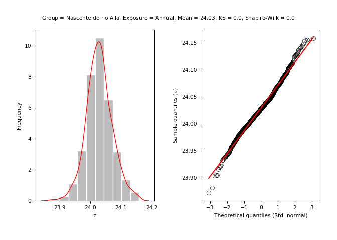
Annual
stats = entrainment.analyze_model(
    model = north_by_year, exposure = "annual", name = x_name
    )
#> ---------------------------------------------------------
#>
#> [Group: Nascente do rio Ailã | Exposure: Annual]
#>
#> Mean = 24.029673997464037
#> Var. = 0.001781775485573474
#> SD = 0.04221108249705845
#>
#> Min. = 23.87209663246515
#> 1st Qu. = 24.00268353458175
#> Median = 24.028647842601398
#> 3rd Qu. = 24.05371460537481
#> Max. = 24.158942185902564
#>
#> Kurtosis = 0.557423923128376
#> Skewness = 0.12169374905078593
#>
#> Kolmogorov-Smirnov test p-value = 0.0
#> Shapiro-Wilks test p-value = 0.00020785177184734493
#>
#> ---------------------------------------------------------
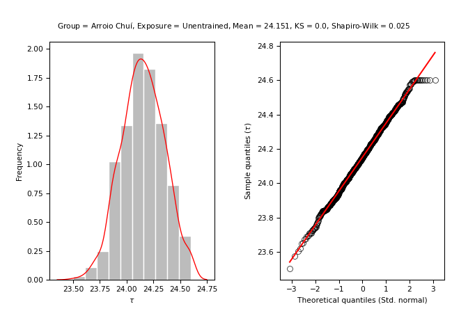
South group (Location: Arroio Chuí) (Latitude: -33.752)
Unentrained (Control)
stats = entrainment.analyze_model(
    model = south_by_season, exposure = "unentrained", name = y_name
    )
#> ---------------------------------------------------------
#>
#> [Group: Arroio Chuí | Exposure: Unentrained]
#>
#> Mean = 24.151103412847707
#> Var. = 0.039084572161572656
#> SD = 0.19769818451764462
#>
#> Min. = 23.5
#> 1st Qu. = 24.017414375153443
#> Median = 24.14923151925353
#> 3rd Qu. = 24.290143195679494
#> Max. = 24.6
#>
#> Kurtosis = -0.2662781596078876
#> Skewness = -0.04667181704412612
#>
#> Kolmogorov-Smirnov test p-value = 0.0
#> Shapiro-Wilks test p-value = 0.02459321916103363
#>
#> ---------------------------------------------------------
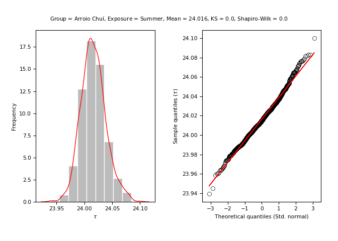
Summer
stats = entrainment.analyze_model(
    model = south_by_season, exposure = "summer", name = y_name
    )
#> ---------------------------------------------------------
#>
#> [Group: Arroio Chuí | Exposure: Summer]
#>
#> Mean = 24.01629854661018
#> Var. = 0.0004917129360020812
#> SD = 0.02217460114640354
#>
#> Min. = 23.939237898632822
#> 1st Qu. = 24.001478216514602
#> Median = 24.014984627202693
#> 3rd Qu. = 24.029971643550606
#> Max. = 24.100225814299897
#>
#> Kurtosis = 0.39990146838379914
#> Skewness = 0.28557138948926486
#>
#> Kolmogorov-Smirnov test p-value = 0.0
#> Shapiro-Wilks test p-value = 0.00014794745948165655
#>
#> ---------------------------------------------------------
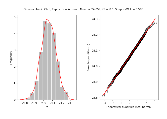
Autumn
stats = entrainment.analyze_model(
    model = south_by_season, exposure = "autumn", name = y_name
    )
#> ---------------------------------------------------------
#>
#> [Group: Arroio Chuí | Exposure: Autumn]
#>
#> Mean = 24.05929683328895
#> Var. = 0.006145459645120493
#> SD = 0.07839298211651662
#>
#> Min. = 23.811796024070986
#> 1st Qu. = 24.006162585268896
#> Median = 24.057382743803288
#> 3rd Qu. = 24.11123992648173
#> Max. = 24.27454364082857
#>
#> Kurtosis = -0.12323675651170385
#> Skewness = 0.02800175398604576
#>
#> Kolmogorov-Smirnov test p-value = 0.0
#> Shapiro-Wilks test p-value = 0.5083744525909424
#>
#> ---------------------------------------------------------
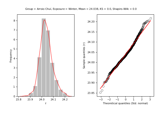
Winter
stats = entrainment.analyze_model(
    model = south_by_season, exposure = "winter", name = y_name
    )
#> ---------------------------------------------------------
#>
#> [Group: Arroio Chuí | Exposure: Winter]
#>
#> Mean = 24.038179750581207
#> Var. = 0.0029098528246764266
#> SD = 0.05394305168116119
#>
#> Min. = 23.851850036956012
#> 1st Qu. = 24.003339438897118
#> Median = 24.033182025434385
#> 3rd Qu. = 24.06865858890189
#> Max. = 24.2171437908377
#>
#> Kurtosis = 0.5440305211695189
#> Skewness = 0.34956426859449286
#>
#> Kolmogorov-Smirnov test p-value = 0.0
#> Shapiro-Wilks test p-value = 2.987544007737597e-07
#>
#> ---------------------------------------------------------
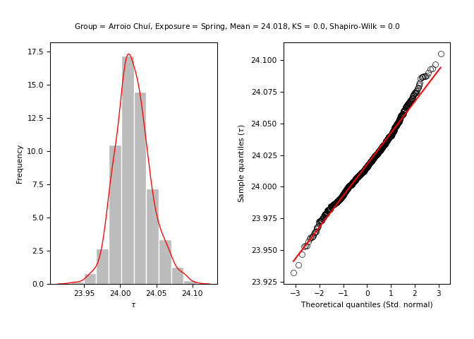
Spring
stats = entrainment.analyze_model(
    model = south_by_season, exposure = "spring", name = y_name
    )
#> ---------------------------------------------------------
#>
#> [Group: Arroio Chuí | Exposure: Spring]
#>
#> Mean = 24.01763571236592
#> Var. = 0.0006076399054779642
#> SD = 0.024650353049763086
#>
#> Min. = 23.932207338966595
#> 1st Qu. = 24.001569417900804
#> Median = 24.015586551801725
#> 3rd Qu. = 24.032190379181696
#> Max. = 24.10501381125711
#>
#> Kurtosis = 0.49878473675342017
#> Skewness = 0.3112905269202585
#>
#> Kolmogorov-Smirnov test p-value = 0.0
#> Shapiro-Wilks test p-value = 6.234316515474347e-06
#>
#> ---------------------------------------------------------
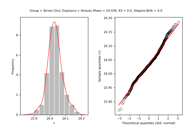
Annual
stats = entrainment.analyze_model(
    model = south_by_year, exposure = "annual", name = y_name
    )
#> ---------------------------------------------------------
#>
#> [Group: Arroio Chuí | Exposure: Annual]
#>
#> Mean = 24.03358038331667
#> Var. = 0.002198528375430825
#> SD = 0.04688846740330531
#>
#> Min. = 23.869188721776947
#> 1st Qu. = 24.00388076427332
#> Median = 24.031453737390798
#> 3rd Qu. = 24.059085689812864
#> Max. = 24.186916928206053
#>
#> Kurtosis = 0.626100024394669
#> Skewness = 0.21178546601162576
#>
#> Kolmogorov-Smirnov test p-value = 0.0
#> Shapiro-Wilks test p-value = 2.19240951082611e-06
#>
#> ---------------------------------------------------------
4. Test the hypothesis
For more information about the values presented, see
scipy.stats.ttest_ind.
Hypothesis statement
Populations residing close to the equator (latitude 0°) (i.e., with greater average insolation) have, on average, a shorter duration/morning circadian period when compared to populations residing near the planet’s poles (i.e., with lower average insolation) (Leocadio-Miguel et al., 2017; Roenneberg et al., 2003).
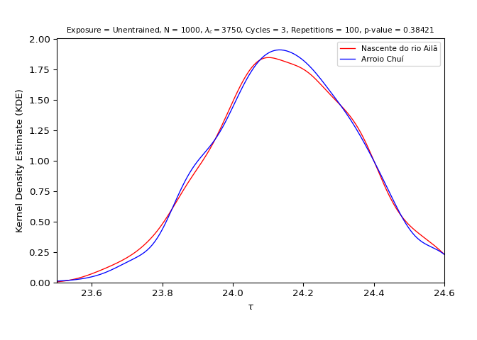
Unentrained (Control)
test = entrainment.test_hypothesis(
    x = north_by_season, y = south_by_season, exposure = "unentrained",
    x_name = x_name, y_name = y_name
    )
#> ---------------------------------------------------------
#>
#> [Group: Nascente do rio Ailã | Exposure: Unentrained]
#>
#> Mean = 24.148469728740682
#> Var. = 0.04081896119474018
#> SD = 0.20203702926627135
#>
#> ---------------------------------------------------------
#>
#> [Group: Arroio Chuí | Exposure: Unentrained]
#>
#> Mean = 24.151103412847707
#> Var. = 0.039084572161572656
#> SD = 0.19769818451764462
#>
#> ---------------------------------------------------------
#>
#> [Groups: Nascente do rio Ailã & Arroio Chuí | Exposure: Unentrained]
#>
#> Variance ratio: 0.04081896119474018 / 0.039084572161572656 = 1.0443752851124402
#> Ratio test: 1.0443752851124402 < 2: TRUE
#>
#> Standard t-test statistic = -0.29448517401917873
#> Standard t-test p-value = 0.38420889134993497
#> Welch’s t-test statistic = -0.29448517401917873
#> Welch’s t-test p-value = 0.384208898556161
#>
#> Cohen's d = 0.013176367180915164
#> Coefficient of determination (R squared) = 0.002072050279476478
#>
#> ---------------------------------------------------------
Summer
test = entrainment.test_hypothesis(
    x = north_by_season, y = south_by_season, exposure = "summer",
    x_name = x_name, y_name = y_name
    )
#> ---------------------------------------------------------
#>
#> [Group: Nascente do rio Ailã | Exposure: Summer]
#>
#> Mean = 24.006999634122447
#> Var. = 0.00012367951240324957
#> SD = 0.01112112909749948
#>
#> ---------------------------------------------------------
#>
#> [Group: Arroio Chuí | Exposure: Summer]
#>
#> Mean = 24.01629854661018
#> Var. = 0.0004917129360020812
#> SD = 0.02217460114640354
#>
#> ---------------------------------------------------------
#>
#> [Groups: Nascente do rio Ailã & Arroio Chuí | Exposure: Summer]
#>
#> Variance ratio: 0.0004917129360020812 / 0.00012367951240324957 = 3.9757024138232446
#> Ratio test: 3.9757024138232446 < 2: FALSE
#>
#> Standard t-test statistic = -11.8478302547822
#> Standard t-test p-value = 1.2045417316886225e-31
#> Welch’s t-test statistic = -11.8478302547822
#> Welch’s t-test p-value = 2.692513130269752e-31
#>
#> Cohen's d = 0.5301162011096661
#> Coefficient of determination (R squared) = 0.0011273452492010561
#>
#> ---------------------------------------------------------
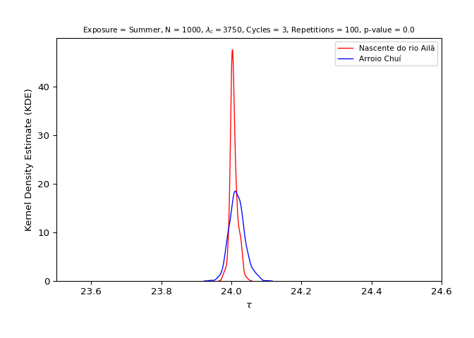
Directional Student’s t-test (Welch’s t-test)
Reject \(H_{0}\) in favour of \(H_{a}\) (\(\text{p-value} = 0.00000\))
Autumn
test = entrainment.test_hypothesis(
    x = north_by_season, y = south_by_season, exposure = "autumn",
    x_name = x_name, y_name = y_name
    )
#> ---------------------------------------------------------
#>
#> [Group: Nascente do rio Ailã | Exposure: Autumn]
#>
#> Mean = 24.006421180918203
#> Var. = 0.00010496412004668206
#> SD = 0.01024519985391608
#>
#> ---------------------------------------------------------
#>
#> [Group: Arroio Chuí | Exposure: Autumn]
#>
#> Mean = 24.05929683328895
#> Var. = 0.006145459645120493
#> SD = 0.07839298211651662
#>
#> ---------------------------------------------------------
#>
#> [Groups: Nascente do rio Ailã & Arroio Chuí | Exposure: Autumn]
#>
#> Variance ratio: 0.006145459645120493 / 0.00010496412004668206 = 58.548193824588274
#> Ratio test: 58.548193824588274 < 2: FALSE
#>
#> Standard t-test statistic = -21.13896654825122
#> Standard t-test p-value = 5.604139343659317e-90
#> Welch’s t-test statistic = -21.138966548251215
#> Welch’s t-test p-value = 5.198081931292546e-83
#>
#> Cohen's d = 0.9458363599883669
#> Coefficient of determination (R squared) = 0.0013431191121989533
#>
#> ---------------------------------------------------------
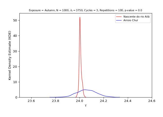
Directional Student’s t-test (Welch’s t-test)
Reject \(H_{0}\) in favour of \(H_{a}\) (\(\text{p-value} = 0.00000\))
Winter
test = entrainment.test_hypothesis(
    x = north_by_season, y = south_by_season, exposure = "winter",
    x_name = x_name, y_name = y_name
    )
#> ---------------------------------------------------------
#>
#> [Group: Nascente do rio Ailã | Exposure: Winter]
#>
#> Mean = 24.006179180043823
#> Var. = 9.583665584921525e-05
#> SD = 0.009789619801055364
#>
#> ---------------------------------------------------------
#>
#> [Group: Arroio Chuí | Exposure: Winter]
#>
#> Mean = 24.038179750581207
#> Var. = 0.0029098528246764266
#> SD = 0.05394305168116119
#>
#> ---------------------------------------------------------
#>
#> [Groups: Nascente do rio Ailã & Arroio Chuí | Exposure: Winter]
#>
#> Variance ratio: 0.0029098528246764266 / 9.583665584921525e-05 = 30.362628984619914
#> Ratio test: 30.362628984619914 < 2: FALSE
#>
#> Standard t-test statistic = -18.448812194563214
#> Standard t-test p-value = 1.3196311333268488e-70
#> Welch’s t-test statistic = -18.448812194563214
#> Welch’s t-test p-value = 1.8316243991266496e-66
#>
#> Cohen's d = 0.8254688010591621
#> Coefficient of determination (R squared) = 0.0009327582812622481
#>
#> ---------------------------------------------------------
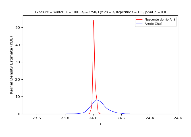
Directional Student’s t-test (Welch’s t-test)
Reject \(H_{0}\) in favour of \(H_{a}\) (\(\text{p-value} = 0.00000\))
Spring
test = entrainment.test_hypothesis(
    x = north_by_season, y = south_by_season, exposure = "spring",
    x_name = x_name, y_name = y_name
    )
#> ---------------------------------------------------------
#>
#> [Group: Nascente do rio Ailã | Exposure: Spring]
#>
#> Mean = 24.005914032779206
#> Var. = 8.699382467490699e-05
#> SD = 0.009327048015042434
#>
#> ---------------------------------------------------------
#>
#> [Group: Arroio Chuí | Exposure: Spring]
#>
#> Mean = 24.01763571236592
#> Var. = 0.0006076399054779642
#> SD = 0.024650353049763086
#>
#> ---------------------------------------------------------
#>
#> [Groups: Nascente do rio Ailã & Arroio Chuí | Exposure: Spring]
#>
#> Variance ratio: 0.0006076399054779642 / 8.699382467490699e-05 = 6.984862520399513
#> Ratio test: 6.984862520399513 < 2: FALSE
#>
#> Standard t-test statistic = -14.05706509060415
#> Standard t-test p-value = 3.5832554548401634e-43
#> Welch’s t-test statistic = -14.05706509060415
#> Welch’s t-test p-value = 3.8125556712327585e-42
#>
#> Cohen's d = 0.6289656236064435
#> Coefficient of determination (R squared) = 0.0009828404429039334
#>
#> ---------------------------------------------------------
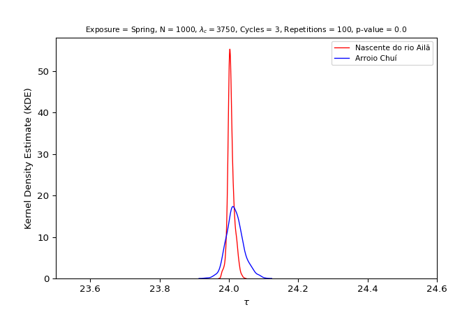
Directional Student’s t-test (Welch’s t-test)
Reject \(H_{0}\) in favour of \(H_{a}\) (\(\text{p-value} = 0.00000\))
Annual
test = entrainment.test_hypothesis(
    x = north_by_year, y = south_by_year, exposure = "annual",
    x_name = x_name, y_name = y_name
    )
#> ---------------------------------------------------------
#>
#> [Group: Nascente do rio Ailã | Exposure: Annual]
#>
#> Mean = 24.029673997464037
#> Var. = 0.001781775485573474
#> SD = 0.04221108249705845
#>
#> ---------------------------------------------------------
#>
#> [Group: Arroio Chuí | Exposure: Annual]
#>
#> Mean = 24.03358038331667
#> Var. = 0.002198528375430825
#> SD = 0.04688846740330531
#>
#> ---------------------------------------------------------
#>
#> [Groups: Nascente do rio Ailã & Arroio Chuí | Exposure: Annual]
#>
#> Variance ratio: 0.002198528375430825 / 0.001781775485573474 = 1.2338975326755137
#> Ratio test: 1.2338975326755137 < 2: TRUE
#>
#> Standard t-test statistic = -1.9570402987776383
#> Standard t-test p-value = 0.02524090110161829
#> Welch’s t-test statistic = -1.9570402987776387
#> Welch’s t-test p-value = 0.02524166355939163
#>
#> Cohen's d = 0.08756529645483169
#> Coefficient of determination (R squared) = 9.076611746535106e-06
#>
#> ---------------------------------------------------------
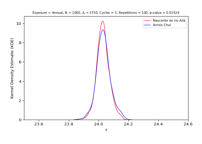
Directional Student’s t-test (Standard t-test)
Reject \(H_{0}\) in favour of \(H_{a}\) (\(\text{p-value} = 0.02524\))